Autosaving every 20 seconds부트스트랩
지난번에 한 구간추정은 이런 과정이였음.
- 모집단으로부터 여러번 임의추출하여 여러개의 표본을 만들고
- 각각의 표본으로부터 추정량의 값인 추정값를 계산하고
- 계산된 추정값들로부터 추정량의 표준편차(또는 분산)을 구하고 + 중심극한정리(CLT)의 이론적 백업을 바탕으로
- 모수 \(\mu\)에 대한 95% 신뢰구간을 제시
- \(\mu\) 는 \(\hat\theta \pm 2SD\)인 구간에 95%확률로 속할 것이다.
- \(\mu - \hat\theta\)의 차이는 95%확률로 \(2SD\)보다 작을 것이다.
하지만 실전에서는 모집단에서 표본은 단 한번 추출함(시간과 비용)
그러면 여러개의 추정값들을 얻을 수 없기에 추정량의 표준편차(\(SD\))를 못 구하는데 어떻게 해야할까?
부트스트랩(bootstrap)을 통해 추정량의 표준편차를 구할 수 있음.
부트스트랩의 목적 : 하나의 샘플만 주어진 상황에서 추정량의 표준편차\(SD\)를 구하여 구간추정을 할 수 있도록 하자.
부트스트랩의 idea : 표본을 모집단처럼 이용하자!
그림
(부트스트랩 과정) 1. 표본으로부터 재추출(resampling)을 통해 재표본(resample)을 만든다. 2. (부트스트랩) 추정치를 구하고 기록한다. 3. 1.2를 여러번 반복한다. 4. 추정량의 분포를 근사하는 경험적 분포와 추정량의 표준편차 \(SD\)를 여러개의 추정치로부터 계산한다.!
(유의해야 할 점) - 재추출(resampling)만 유의하면 된다. - 재추출은 표본으로부터 복원추출 - 표본과 재표본의 크기는 같아야 함.
Bootstrap 실습
모집단 생성
모집단에서 하나의 확률표본만 있다고 가정
표본지지율은 ?
부트스트랩 ㄱㄱㅆ
- 부트스트랩 과정 recap
- 표본으로부터 복원추출하여 크기=n인 재표본을 생성
- 생성된 재표본으로부터 추정량 계산
- 이전 과정2개를 반복하여 여러개의 추정값들 계산
- 추정값들의 분포가 추정량의 분포와 거의 비슷하다!
- 추정량의 분산도 여기서 구하면 되겠지?
B = 1000 #부트스트랩 모의실험 횟수. 추정값들의 갯수와 동일

bootstrap_estimates = pd.DataFrame({"resample_estimate":np.zeros(B)}) # B개의 추정치를 저장할 데이터프레임 확보

for i in np.arange(B):
    resample = np.random.choice(one_sample,n,replace=True)
    bootstrap_estimates.loc[i,"resample_estimate"] = resample.mean()
bootstrap_estimates.head(10)| resample_estimate | |
|---|---|
| 0 | 0.532 |
| 1 | 0.504 |
| 2 | 0.478 |
| 3 | 0.491 |
| 4 | 0.497 |
| 5 | 0.512 |
| 6 | 0.508 |
| 7 | 0.523 |
| 8 | 0.507 |
| 9 | 0.484 |
여러번 sampling vs 여러번 resampling(부트스트랩)
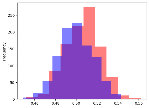
\(SD\)구하기
- \(SD\)는 \(Std(\hat\theta)\)를 근사적으로 구한 값이라 하자.(이전에는 sampling을 여러번해서 구했었음)
참고 - 여러번 sampling한 추정량의 분포로부터 구한 SD는?
- 매우매우 유사하다.
참고 - 중심극한 정리에 의한 이론적인 추정량의 분산은?
\[ \begin{aligned} &Var(\hat\theta) = \frac{\sigma^2}{n} \\ &Std(\hat\theta) = \sqrt{\frac{\sigma^2}{n}} \\ \end{aligned} \]
- 매우매우 유사하다.
Bootstrap을 사용한 구간추정
SD활용
Percentile 사용
신뢰구간 해석
- 95%의 확률로 신뢰구간이 모수를 포함한다. (\(\hat\theta\)가 확률변수, \(\theta\)는 고정된 상수,신뢰구간이 바뀐다. 고전적인 통계의 관점)
- 95%의 확률로 모수가 신뢰구간에 포함된다. (\(\theta\)가 확률변수, \(\hat\theta\)는 고정된 상수,신뢰구간은 고정.베이지안 관점)
세부적으로 이렇게 적을 수 있지만 사실 차이가 이해하기 어려우므로 95% 신뢰구간에 모수가 포함되었을 가능성이 95%라 생각해도 큰 문제는 없다.
예제 : 중앙값의 신뢰구간 구하기
| 자전거번호 | 대여일시 | 대여 대여소번호 | 대여 대여소명 | 대여거치대 | 반납일시 | 반납대여소번호 | 반납대여소명 | 반납거치대 | 이용시간 | 이용거리 | |
|---|---|---|---|---|---|---|---|---|---|---|---|
| 0 | SPB-17003 | 2019-09-28 16:10:55 | 368 | SK 서린빌딩 앞 | 4 | 2019-09-28 17:03:32 | 2002 | 노들역 1번출구 | 14 | 52 | 8940.0 |
| 1 | SPB-14405 | 2019-09-28 16:48:16 | 2024 | 상도역 1번출구 | 3 | 2019-09-28 17:03:44 | 2002 | 노들역 1번출구 | 18 | 15 | 1910.0 |
| 2 | SPB-18431 | 2019-09-28 16:59:54 | 2002 | 노들역 1번출구 | 10 | 2019-09-28 17:03:57 | 2002 | 노들역 1번출구 | 10 | 2 | 30.0 |
| 3 | SPB-04853 | 2019-09-28 15:31:49 | 207 | 여의나루역 1번출구 앞 | 32 | 2019-09-28 17:10:12 | 2002 | 노들역 1번출구 | 19 | 98 | 9610.0 |
| 4 | SPB-11122 | 2019-09-28 15:35:41 | 207 | 여의나루역 1번출구 앞 | 14 | 2019-09-28 17:10:37 | 2002 | 노들역 1번출구 | 18 | 90 | 9450.0 |
| ... | ... | ... | ... | ... | ... | ... | ... | ... | ... | ... | ... |
| 407584 | SPB-24072 | 2019-09-12 08:56:34 | 240 | 문래역 4번출구 앞 | 9 | 2019-09-12 09:03:37 | 99999 | 영남단말기정비 | 2 | 6 | 720.0 |
| 407585 | SPB-16130 | 2019-09-18 10:13:09 | 99999 | 영남단말기정비 | 1 | 2019-09-18 11:38:30 | 99999 | 영남단말기정비 | 1 | 85 | 40.0 |
| 407586 | SPB-03728 | 2019-09-25 08:00:28 | 2183 | 동방1교 | 7 | 2019-09-25 08:54:02 | 99999 | 영남단말기정비 | 5 | 53 | 12910.0 |
| 407587 | SPB-08928 | 2019-09-30 07:49:27 | 2183 | 동방1교 | 10 | 2019-09-30 09:42:27 | 99999 | 영남단말기정비 | 7 | 2 | 0.0 |
| 407588 | SPB-06988 | 2019-09-30 09:58:43 | 99999 | 영남단말기정비 | 5 | 2019-09-30 13:01:26 | 99999 | 영남단말기정비 | 5 | 182 | 10.0 |
407589 rows × 11 columns
| 이용시간 | 이용거리 | |
|---|---|---|
| 0 | 52 | 8940.0 |
| 1 | 15 | 1910.0 |
| 2 | 2 | 30.0 |
| 3 | 98 | 9610.0 |
| 4 | 90 | 9450.0 |
| ... | ... | ... |
| 407584 | 6 | 720.0 |
| 407585 | 85 | 40.0 |
| 407586 | 53 | 12910.0 |
| 407587 | 2 | 0.0 |
| 407588 | 182 | 10.0 |
407589 rows × 2 columns
| 이용시간 | 이용거리 | |
|---|---|---|
| count | 407589.000000 | 407589.000000 |
| mean | 30.156827 | 4253.336228 |
| std | 32.065934 | 5782.673901 |
| min | 1.000000 | 0.000000 |
| 25% | 8.000000 | 1200.000000 |
| 50% | 18.000000 | 2380.000000 |
| 75% | 43.000000 | 5130.000000 |
| max | 2479.000000 | 153490.000000 |
| 이용시간 | 이용거리 | |
|---|---|---|
| 50771 | 25 | 1830.0 |
| 179510 | 20 | 3670.0 |
| 167844 | 8 | 1180.0 |
| 244482 | 3 | 210.0 |
| 102805 | 9 | 1330.0 |
| 330458 | 15 | 3090.0 |
| 91162 | 3 | 730.0 |
| 22447 | 6 | 1940.0 |
| 348599 | 16 | 1350.0 |
| 387639 | 15 | 2270.0 |
| 이용시간 | 이용거리 | |
|---|---|---|
| count | 1000.000000 | 1000.000000 |
| mean | 28.150000 | 3923.110000 |
| std | 28.664598 | 4723.684348 |
| min | 1.000000 | 0.000000 |
| 25% | 8.000000 | 1247.500000 |
| 50% | 18.000000 | 2345.000000 |
| 75% | 41.000000 | 5040.000000 |
| max | 321.000000 | 70890.000000 |
B = 1000
n = 1000

bootstrap_estimates = pd.DataFrame({"time_estimate":np.zeros(B),"distance_estimate":np.zeros(B)})
for i in np.arange(B):
    resample = one_sample.sample(n=n,replace=True,random_state = i)
    bootstrap_estimates.loc[i,"time_estimate"] = np.median(resample["이용시간"])
    bootstrap_estimates.loc[i,"distance_estimate"] = np.median(resample["이용거리"])
bootstrap_estimates.head(10)| time_estimate | distance_estimate | |
|---|---|---|
| 0 | 18.0 | 2305.0 |
| 1 | 17.0 | 2330.0 |
| 2 | 18.0 | 2365.0 |
| 3 | 18.0 | 2410.0 |
| 4 | 19.0 | 2330.0 |
| 5 | 18.0 | 2355.0 |
| 6 | 17.0 | 2310.0 |
| 7 | 17.0 | 2320.0 |
| 8 | 17.0 | 2315.0 |
| 9 | 18.0 | 2375.0 |
lower_bound = float(np.quantile(bootstrap_estimates[["time_estimate"]],0.025))
upper_bound = float(np.quantile(bootstrap_estimates[["time_estimate"]],0.975))
lower_bound,upper_bound
(16.5, 20.0)lower_bound = float(np.quantile(bootstrap_estimates["distance_estimate"],0.025))
upper_bound = float(np.quantile(bootstrap_estimates["distance_estimate"],0.975))
lower_bound,upper_bound(2180.0, 2530.25)n = 1000 # 표본의 크기
one_sample = bike2.sample(n=n, replace=False, random_state=13312)
one_sample
B = 1000 # 붓스트랩 모의실험의 횟수
bootstrap_estimates = pd.DataFrame({'time_boot':np.zeros(B), 'distance_boot':np.zeros(B)})
for i in np.arange(B):
boot_sample = one_sample.sample(n=n, replace=True, random_state=i)
bootstrap_estimates.loc[i,'time_boot'] = np.median(boot_sample.time)
bootstrap_estimates.loc[i,'distance_boot'] = np.median(boot_sample.distance)
bootstrap_estimates | time_boot | distance_boot | |
|---|---|---|
| 0 | 18.0 | 2305.0 |
| 1 | 17.0 | 2330.0 |
| 2 | 18.0 | 2365.0 |
| 3 | 18.0 | 2410.0 |
| 4 | 19.0 | 2330.0 |
| ... | ... | ... |
| 995 | 17.5 | 2305.0 |
| 996 | 19.0 | 2360.0 |
| 997 | 19.0 | 2315.0 |
| 998 | 17.0 | 2320.0 |
| 999 | 19.0 | 2375.0 |
1000 rows × 2 columns